
There are already many open-source tools available out there for analyzing and creating factor-based trading strategies. Among those, perhaps the most popular one is Alphalens by the Quantopian team, which has had a pivotal role in the career of thousands of aspiring Quants like myself looking to learn industry-standard techniques for factor analysis.
As a personal project, and with the objective to better understand these techniques, I did my own implementation (and sometimes interpretation) of some of the features of Alphalens using my favorite engine LEAN and QuantConnect. I am now sharing this product to help QuantConnect users perform factor research and strategy backtesting in their favorite platform. You will find the full product at the end of this article, which can be directly cloned into your QuantConnect account.
I would like to add here that even though the features in this product look very similar to those in Alphalens, I did not use (or look at) any of their open-source code to build it.
I believe factor investing is a very interesting area to explore within financial trading and this is my contribution to the community. I hope this product will improve over time and strongly encourage questions and suggestions!
This article consists of the following parts:
- A brief introduction to factor investing.
- Case Study – Factor Research: How to use the research tools to analyze a long-short equity strategy based on the combination of two factors (momentum and volatility)
- Case Study – Risk Research: Explore the influence that some external risk factors might have on our strategy.
- Case Study – Backtesting Algorithm: After completing the research phase, we will show how to seamlessly move the strategy to the algorithm to test it against historical data, including slippage and commission modeling.
About Factor Investing
Factor investing is a popular investment approach consisting of finding quantifiable attributes of companies that are associated with their future performance for a given period of time.
A Matter Of Relative Performance
The general hypothesis behind this type of strategy is that it is possible to rank stocks based on certain factors that successfully separate winners from losers, and then construct a large portfolio that goes long the top stocks and short the bottom ones profiting from the spread between their future returns.
The concept of winners and losers here refers to the performance of the stocks relative to each other, not in absolute terms. This means that even if all stocks go up or down at the same time, we can still profit if we are able to segregate the ones that do better than others.
This concept makes factor investing very attractive since it is not about predicting individual stocks or specific moves up or down, but rather finding groups of assets that on average perform consistently above others.
What Makes A Factor
In principle, a factor can be anything that we can quantify for a company using the data available to us at that moment in time. We can calculate factors based on fundamentals (revenues, earnings, future growth, return on equity, profit margins, etc.), historical pricing and volume data (momentum, volatility, liquidity, technical indicators, statistical factors, etc.), or alternative data (news, market sentiment, etc.).
Perhaps a most interesting question would be what makes a “good” factor. The short answer is a factor that proves to be a consistent driver of future returns in either direction across many stocks. This article will present a series of standard statistical techniques commonly used to assess the quality of factors.
In any case, most factor-based strategies will include multiple factors that are uncorrelated with each other and when combined into one model help explain the performance of the stocks better than any individual factor alone. One way of doing this, as we will show later, is by creating a factor from some linear combination of other factors. Ultimately, Machine Learning can be really helpful to identify the relative importance of each factor and find a meaningful, low-bias combination of them.
Cyclical Performance
Finding factors that always work through any economic period and market context is not realistic. Instead, factors tend to move between cycles of overperformance and underperformance over time. Factor timing is incredibly hard, but at least we can try to better understand the drivers behind these periods. Risk analysis will help us with this task which essentially consists of finding external factors that are somehow correlated with our factors in order to explain, and perhaps even anticipate, these performance cycles.
Market Neutral
These strategies are commonly executed using a large number of stocks on each side (long-short), resulting in a market-neutral (zero beta) portfolio whose performance will solely depend on the quality of the ranking system.
Case Study – Factor Research
This section corresponds to the FactorAnalysis class whose purpose is to build a long-short portfolio based on statistically significant factors. The Notebook also contains detailed step-by-step instructions.
For this first version, we have focused on factors created using historical price and volume data simply because we found historical fundamental data (when requested for many tickers and years) is still too computationally expensive to do in QuantConnect. Once this is improved we will work to add fundamental factors to the product.
Initialize Data
The first thing we need to do is to add our start and end dates and initialize the FactorAnalysis class by passing a list of tickers. We need to provide a manual list of tickers because at the time of this article QuantConnect does not offer a dynamic universe in the research environment (looking forward to that!). In our example, we’re using a list with all the SP500 constituents as of Q4 2020.
# select start and end date for analysis
startDate = datetime(2017, 1, 1)
endDate = datetime(2020, 10, 1)
# initialize factor analysis
factorAnalysis = FactorAnalysis(qb, tickers, startDate, endDate, Resolution.Daily)
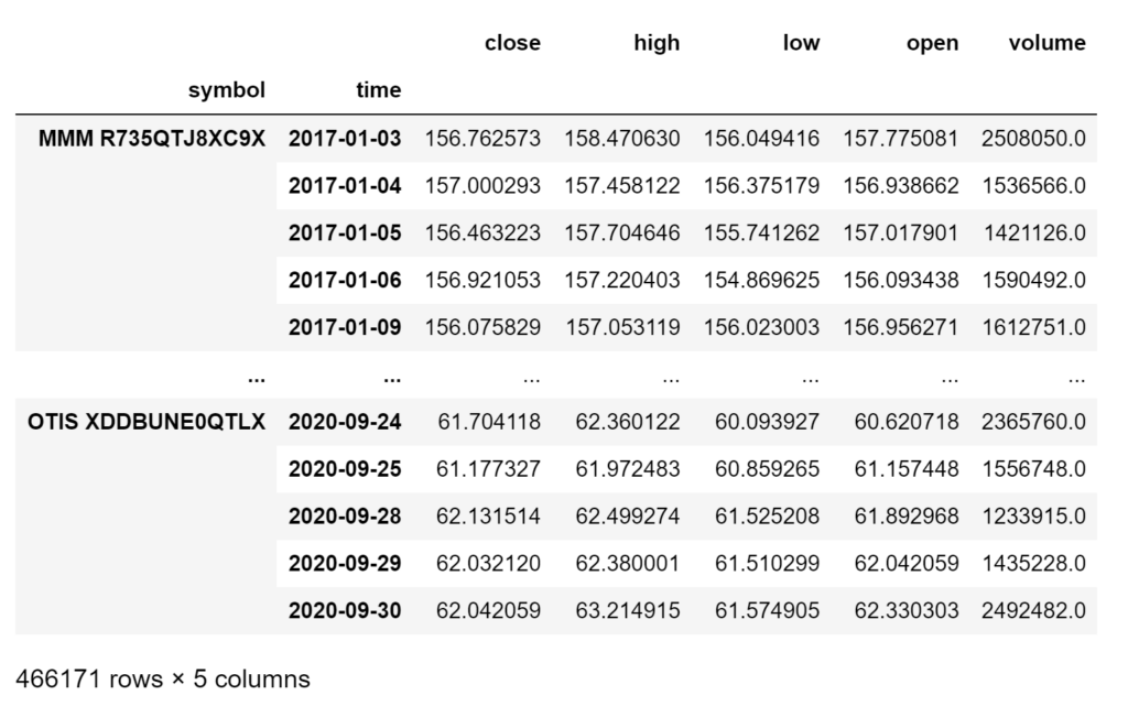
This is going to create a MultiIndex Dataframe with the historical OHLCV daily data needed for analysis.
factorAnalysis.ohlcvDf
Create Factors
Now we are going to create two very simple factors, Momentum and Volatility, using the CustomFactor function as follows.
# example of calculating multiple factors using the CustomFactor function

from scipy.stats import skew, kurtosis

def CustomFactor(x):

    '''
    Description:
        Applies factor calculations to a SingleIndex DataFrame of historical data OHLCV by symbol
    Args:
        x: SingleIndex DataFrame of historical OHLCV data for each symbol
    Returns:
        The factor value for each day
    '''

    try:
        # momentum factor --------------------------------------------------------------------------
        closePricesTimeseries = x['close'].rolling(252) # create a 252 day rolling window of close prices
        returns = x['close'].pct_change().dropna() # create a returns series
        momentum = closePricesTimeseries.apply(lambda x: (x[-1] / x[-252]) - 1)

        # volatility factor ------------------------------------------------------------------------
        volatility = returns.rolling(252).apply(lambda x: np.nanstd(x, axis = 0))

        # get a dataframe with all factors as columns --------------------------------------------
        factors = pd.concat([momentum, volatility], axis = 1)

    except BaseException as e:
        factors = np.nan

    return factors
What’s going on there?
- Under the hood, this function gets applied to the OHLCV DataFrame grouped by symbol. That means we can perform calculations for each symbol using any of the OHLCV columns in the grouped ‘x’ DataFrame.
- We want to calculate factors in a rolling fashion so we get a value for each day that is calculated using data up until that day and including that day. By doing this we assume that in backtesting (and live trading) the calculations and trading decisions happen after the market close and before the next open.
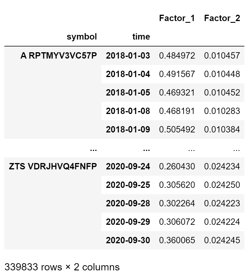
- Finally, we concatenate the factors so we get the resulting DataFrame with one column per factor.
# example of a multiple factors
factorsDf = factorAnalysis.GetFactorsDf(CustomFactor)

factorsDf
In order to standardize the data, we apply winsorization and z-score normalization. We won’t go over that here so please refer to the Notebook for more information on this.
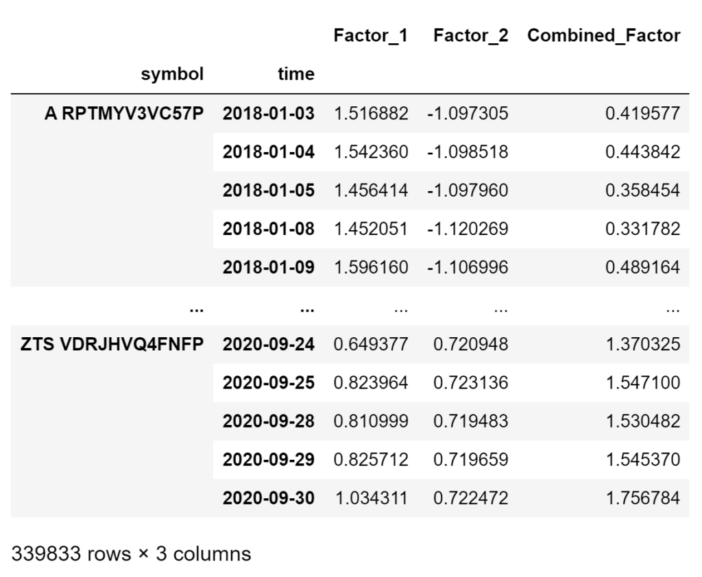
We have two single factors and we want to combine them into one factor that is some linear combination of the two. We do this using the combinedFactorWeightsDict that takes the factor names and the weights. Note how we could reverse the effect of a factor by assigning a negative weight here. In this example, we will just sum the two.
# dictionary containing the factor name and weights for each factor
combinedFactorWeightsDict = {'Factor_1': 1, 'Factor_2': 1}
#combinedFactorWeightsDict = None # None to not add a combined factor when using single factors

finalFactorsDf = factorAnalysis.GetCombinedFactorsDf(standardizedFactorsDf, combinedFactorWeightsDict)

finalFactorsDf
Create Quantiles And Add Forward Returns
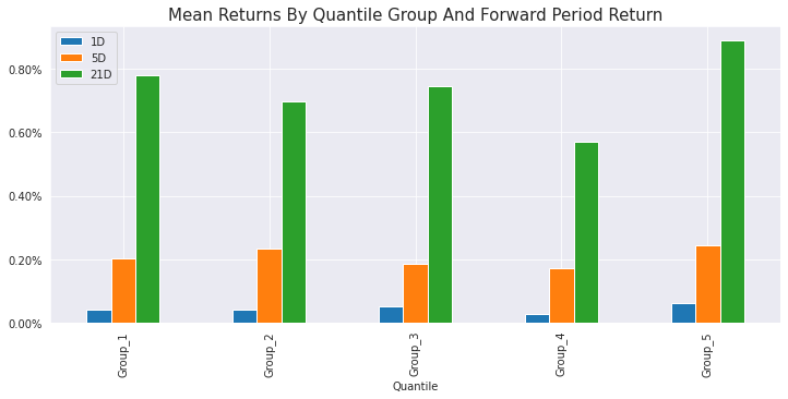
It is time to create our factor quantiles and calculate forward returns in order to assess the relationship between the two.
# inputs for forward returns calculations
forwardPeriods = [1, 5, 21] # choose periods for forward return calculations

# inputs for quantile calculations
factor = 'Combined_Factor' # choose a factor to create quantiles
q = 5 # choose the number of quantile groups to create

factorQuantilesForwardReturnsDf = factorAnalysis.GetFactorQuantilesForwardReturnsDf(finalFactorsDf, field, forwardPeriods, factor, q)

factorQuantilesForwardReturnsDf
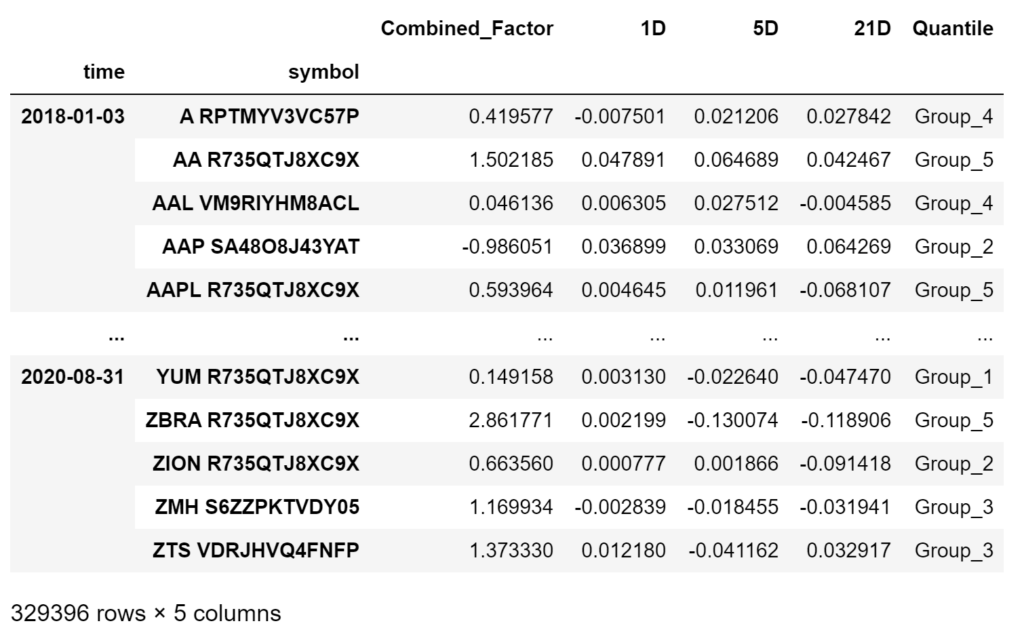
- In order to calculate forward returns, we need to choose the different periods we want to get. In this example, we are calculating the 1, 5, and 21 forward returns based on Close prices.
- We select the factor we want to use for the quantiles and how many quantile groups we want to create. We are using the
Combined_Factorand 5 quintiles here.
Let’s have a look at the mean returns.
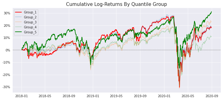
The next step is to visualize the cumulative returns from each quintile over time. In order to do that, we are going to group by quintile every day and calculate the return for each quintile/day by either using equal-weighting (mean) or factor-based weighting (weight the return of each stock in the quintile by its factor value).
forwardPeriod = 1 # choose the forward period to use for returns
weighting = 'mean' # mean/factor

returnsByQuantileDf = factorAnalysis.GetReturnsByQuantileDf(factorQuantilesForwardReturnsDf, forwardPeriod, weighting)

returnsByQuantileDf
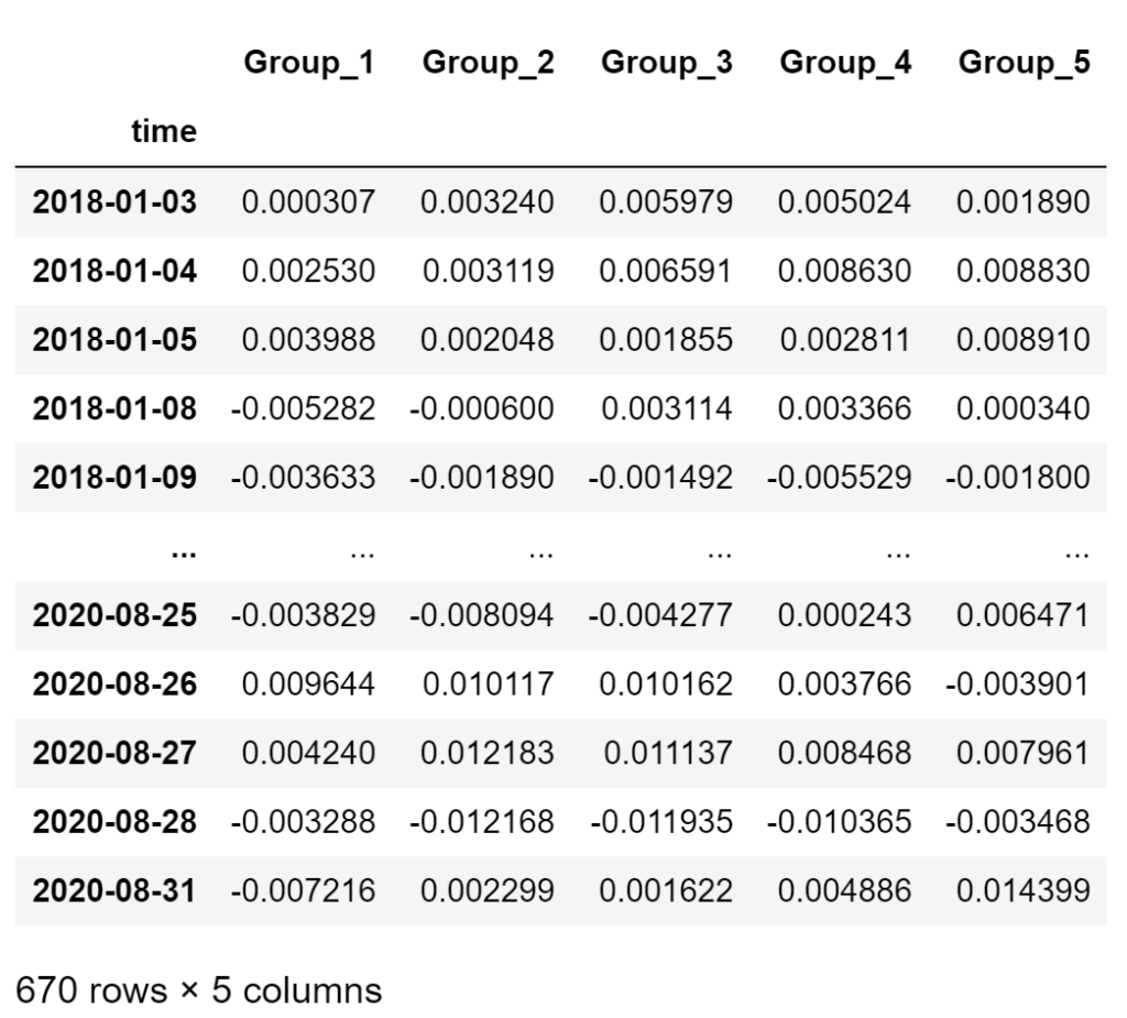
Here we are ideally looking for returns series that deviate from each other in the direction of the quintiles order (top quintile going up while bottom quintile going down).
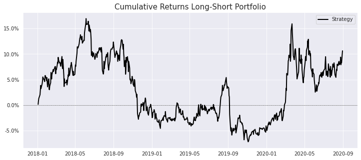
Create a Long-Short Portfolio
We are finally in a position to construct a portfolio that exploits the spread between the top and bottom quintiles. In order to do this, we need to select two quintiles and provide some weighting that we want to apply to each of them using the portfolioWeightsDict. This allows for some flexibility in the way we create the portfolio as we can give more or less weight to one of the quintiles.
# dictionary containing the quintile group names and portfolio weights for each
portfolioWeightsDict = {'Group_5': 1, 'Group_1': -1}

portfolioLongShortReturnsDf = factorAnalysis.GetPortfolioLongShortReturnsDf(returnsByQuantileDf, portfolioWeightsDict)

portfolioLongShortReturnsDf
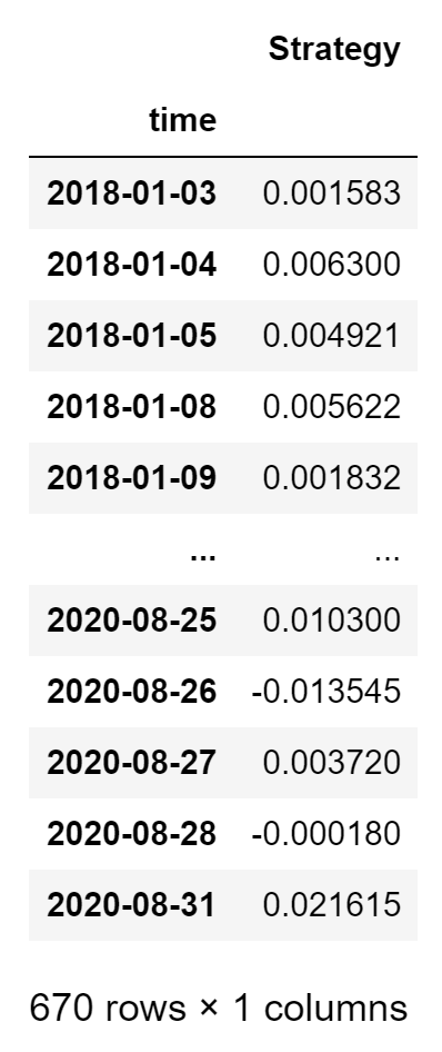
And the plot!
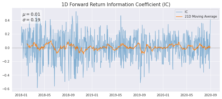
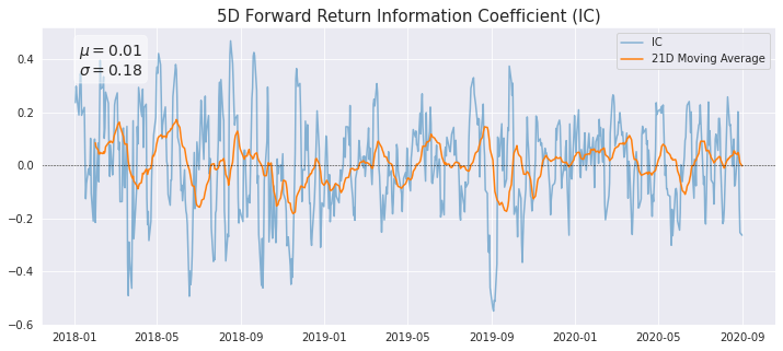
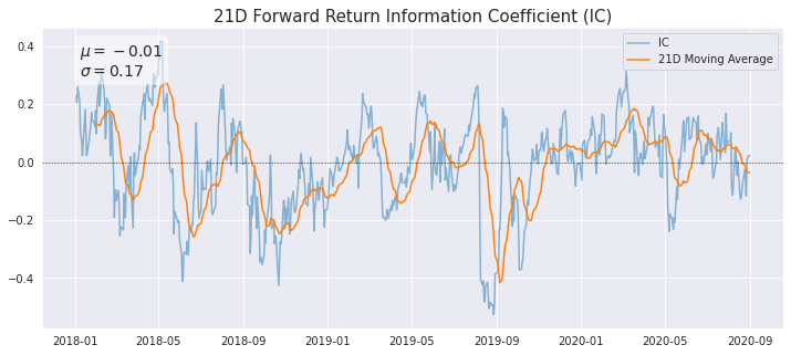
Spearman Rank Correlation Coefficient
A standard way of assessing the degree of correlation between our factor and forward returns is the Spearman Rank Correlation (Information Coefficient).
The Spearman Rank Correlation measures the strength and direction of the association between two ranked variables. It is the non-parametric version of the Pearson correlation and focuses on the monotonic relationship between two variables rather than their linear relationship. Below we plot the daily IC between the factor values and each forward period return, along with a 21-day moving average.
factorAnalysis.PlotIC(factorQuantilesForwardReturnsDf)
Case Study – Risk Research
This section corresponds to the RiskAnalysis class whose purpose is to discover what risk factors our strategy is exposed to and to what degree. As we will see below in more detail, these external factors can be any time series of returns that our portfolio could have some exposure to. Some popular risk factors are provided here (Fama-French Five Factors, Industry Factors), but the user can easily test any other by passing its time series of returns. The Notebook also contains detailed step-by-step instructions.
Initialize Data
Let’s initialize the RiskAnalysis class.
# initialize risk analysis
riskAnalysis = RiskAnalysis(qb)
After initializing the RiskAnalysis class, we get two datasets with classic risk factors:
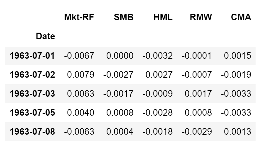
- Fama-French 5 Factors: Historical daily returns of Market Excess Return (Mkt-RF), Small Minus Big (SMB), High Minus Low (HML), Robust Minus Weak (RMW), and Conservative Minus Aggressive (CMA).
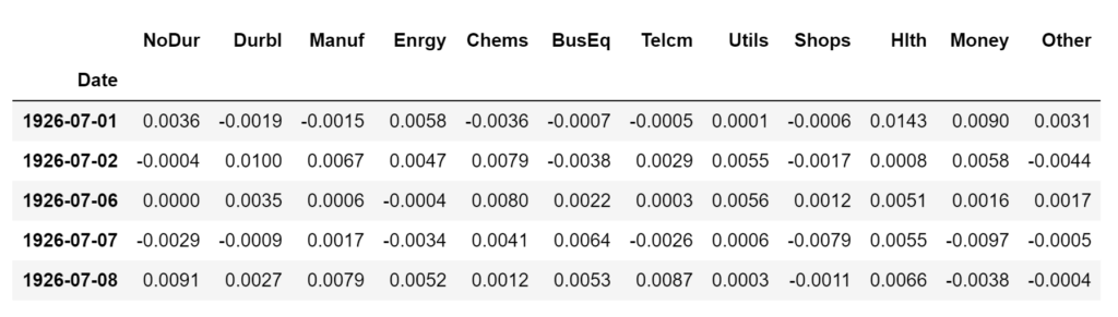
- 12 Industry Factors: Consumer Nondurables (NoDur), Consumer durables (Durbl), Manufacturing (Manuf), Energy (Enrgy), Chemicals (Chems), Business Equipment (BusEq), Telecommunications (Telcm), Utilities (Utils), Wholesale and Retail (Shops), Healthcare (Hlth), Finance (Money), Other (Other)
Visit this site for more factor datasets to add to this analysis.
# fama-french 5 factors
riskAnalysis.ffFiveFactorsDf.head()
# 12 industry factors
riskAnalysis.industryFactorsDf.head()
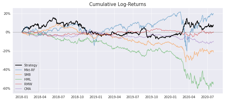
Let’s take a look at the cumulative returns of our long-short strategy together with the returns of the Fama-French 5 Factors.
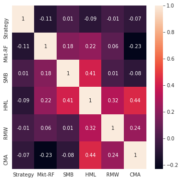
We can visualize the correlations between the risk factors and our strategy returns.
# plot correlation matrix
factorAnalysis.PlotFactorsCorrMatrix(combinedReturnsDf))
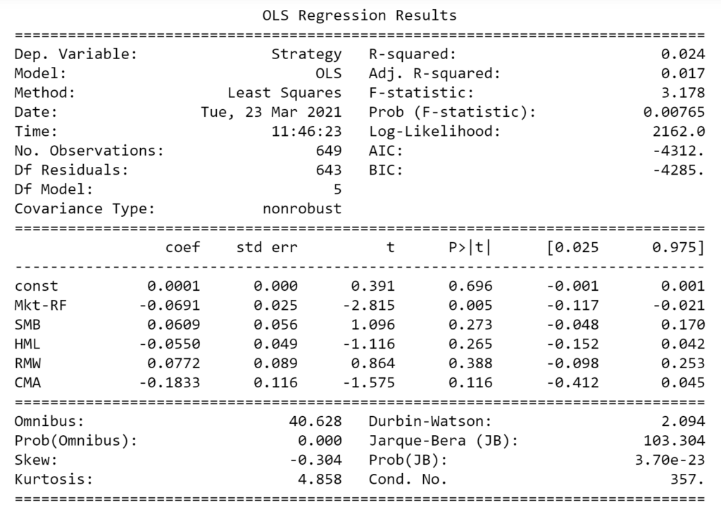
Run Regression Analysis
- Fit a Regression Model to the data to analyze linear relationships between our strategy returns and the external risk factors.
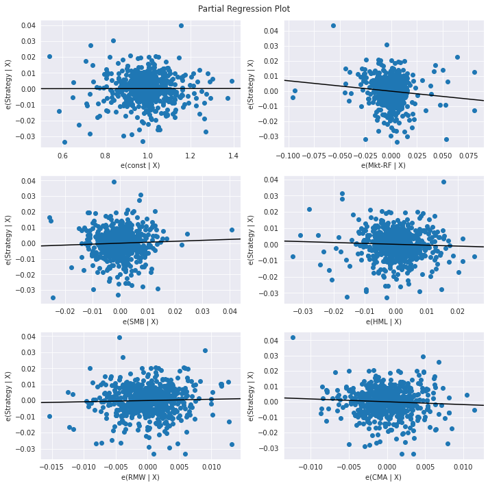
- Partial Regression plots. When performing multiple linear regression, these plots are useful in analyzing the relationship between each independent variable and the response variable while accounting for the effect of all the other independent variables present in the model. Calculations are as follows (Wikipedia):
- Compute the residuals of regressing the response variable against the independent variables but omitting Xi.
- Compute the residuals from regressing Xi against the remaining independent variables.
- Plot the residuals from (1) against the residuals from (2).
riskAnalysis.PlotRegressionModel(combinedReturnsDf, dependentColumn = 'Strategy')
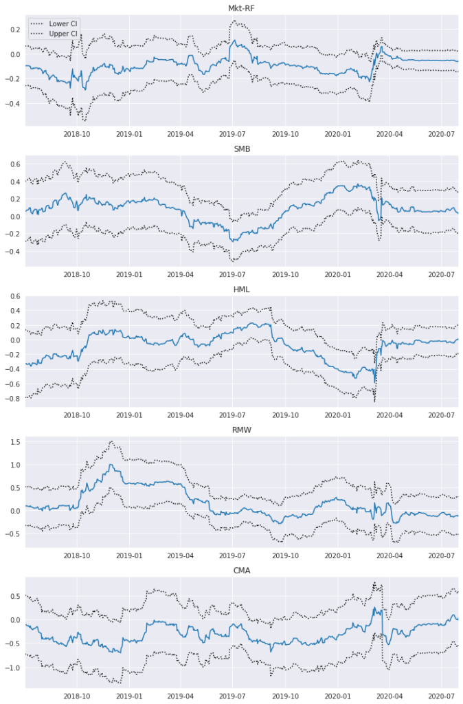
Plot Rolling Regression Coefficients
The above relationships are not static through time, therefore it is useful to visualize how these coefficients behave over time by running a Rolling Regression Model (with a given lookback period).
riskAnalysis.PlotRollingRegressionCoefficients(combinedReturnsDf, dependentColumn = 'Strategy', lookback = 126)
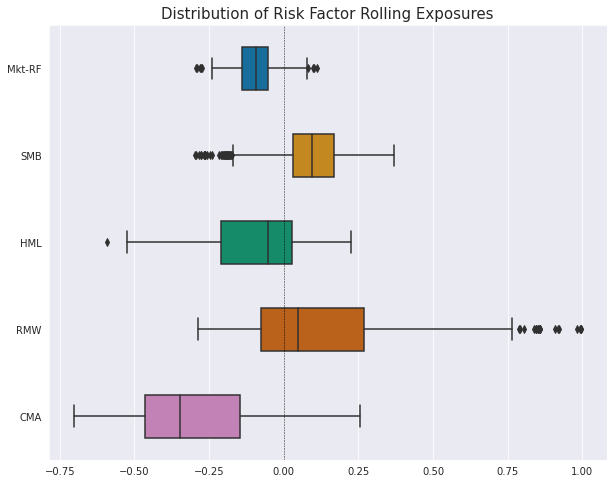
Plot Distribution Of Rolling Exposures
We can now visualize the historical distributions of the rolling regression coefficients in order to get a better idea of the variability of the data.
riskAnalysis.PlotBoxPlotRollingFactorExposure(combinedReturnsDf, dependentColumn = 'Strategy', lookback = 126)
Case Study – Backtesting Algorithm
The purpose of the research process illustrated above is purely to determine if there is a significant relationship between our factors and the future returns of those stocks. That means the cumulative returns we saw are not realistic and they assumed daily rebalancing of hundreds of stocks without accounting for any slippage or commissions.
In order to test how this strategy would have performed historically, we need to run a proper backtest, and for that, we have to move from the Research Notebook to the Algorithm Framework.
Below I will explain the most important features and scripts of this part of the product.
Algorithm Framework – main.py
The main.py script includes the following user-defined inputs worth mentioning.
# date rule for rebalancing our portfolio by updating long-short positions based on factor values
rebalancingFunc = Expiry.EndOfMonth

# number of stocks to keep for factor modelling calculations
nStocks = 100

# number of positions to hold on each side (long/short)
positionsOnEachSide = 20

# lookback for historical data to calculate factors
lookback = 252

# select the leverage factor
leverageFactor = 1
- We first need to select how often we want to rebalance the portfolio (i.e. recalculate all factors and portfolio weights). Here you can choose among a number of date rules such as
Expiry.EndOfMonth - At every rebalancing, the algorithm will create a dynamic universe of stocks based on
DollarVolumeandMarketCapthat will be used to calculate the factors on (nStocks) and ultimately select the top and bottom stocks to trade (positionsOnEachSide). - Finally, we need to decide how much historical data we want for our factors calculations using
lookback - There is also a
leverageFactorparameter that can be used to modify the account leverage.
Algorithm Framework – classSymbolData.py
The Backtesting Algorithm has been designed to make it easy to quickly add and remove the factors previously analyzed in the notebook. We only need to add the function that calculates the factor to the SymbolData class. For example, have a look at how we add the Momentum and Volatility factors from before.
def CalculateMomentum(self, history):

    closePrices = history.loc[self.Symbol]['close']
    momentum = (closePrices[-1] / closePrices[-252]) - 1

    return momentum

def CalculateVolatility(self, history):

    closePrices = history.loc[self.Symbol]['close']
    returns = closePrices.pct_change().dropna()
    volatility = np.nanstd(returns, axis = 0)

    return volatility
You can add as many functions as you want and then simply include them or exclude them from the strategy by simply commenting out the function call here. Note how there are a few functions for other factors that we commented out to leave out of the strategy.
def CalculateFactors(self, history, fundamentalDataBySymbolDict):

    self.fundamentalDataDict = fundamentalDataBySymbolDict[self.Symbol]
    self.momentum = self.CalculateMomentum(history)
    self.volatility = self.CalculateVolatility(history)
    #self.skewness = self.CalculateSkewness(history)
    #self.kurt = self.CalculateKurtosis(history)
    #self.distanceVsHL = self.CalculateDistanceVsHL(history)
    #self.meanOvernightReturns = self.CalculateMeanOvernightReturns(history)
And at the end, we just need to add the chosen factors to the property factorsList
@property
def factorsList(self):
    technicalFactors = [self.momentum, self.volatility]
Algorithm Framework – HelperFunctions.py
In the Research Notebook we could only add factors created using OHLCV data for the reasons already stated above. However, the Backtesting Algorithm allows adding fundamental factors very easily by using the GetFundamentalDataDict function. As you can see below, we create a dictionary containing the fundamental ratio and its desired direction in the model (1 for a positive effect or -1 for a negative one). For a list of all the fundamental data available in QuantConnect please refer to this page https://www.quantconnect.com/docs/data-library/fundamentals
# dictionary of symbols containing factors and the direction of the factor (1 for sorting descending and -1 for sorting ascending)
fundamentalDataBySymbolDict[x.Symbol] = {
                                         #fundamental.ValuationRatios.BookValuePerShare: 1,
                                         #fundamental.FinancialStatements.BalanceSheet.TotalEquity.Value: -1,
                                         #fundamental.OperationRatios.OperationMargin.Value: 1,
                                         #fundamental.OperationRatios.ROE.Value: 1,
                                         #fundamental.OperationRatios.TotalAssetsGrowth.Value: 1,
                                         #fundamental.ValuationRatios.NormalizedPERatio: 1,
                                         #fundamental.ValuationRatios.PBRatio: -1,
                                         #fundamental.OperationRatios.TotalDebtEquityRatio.Value: -1,
                                         #fundamental.ValuationRatios.FCFRatio: -1,
                                         #fundamental.ValuationRatios.PEGRatio: -1,
                                         #fundamental.MarketCap: 1,
                                         }
Finally, very much like we did in the Research Notebook, in the Backtesting Algorithm we can also give different weights to each factor to create a combined factor. We do that using the GetLongShortLists function in the HelperFunctions.py script as per below.
normFactorsDf['combinedFactor'] = normFactorsDf['Factor_1'] * 1 + normFactorsDf['Factor_2'] * 1
Clone The Algorithm
And that was it! Now you can clone the below algorithm into your QuantConnect account and start playing with the different features yourself. The algorithm also has a number of interesting backtesting charts such as Drawdown and Total Portfolio Exposure %, so remember to activate those on the Select Chart box (top right corner of backtesting page).
FACTOR INVESTING SYSTEM (Research & Algorithm)
Do you have a strategy of your own that you would like to backtest and automate? Get in touch to learn more about our consulting services!